Numerical Solution of the Diffusion Equation with No-Flux Boundary Conditions

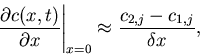
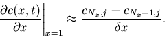
For no-flux boundary conditions, we want $\left. \frac{\partial c}{\partial x} \right\vert _{x=0} = \left. \frac{\partial c}{\partial x} \right\vert _{x=1} = 0$. Notice that

$$\left. \frac{\partial c(x,t)}{\partial x} \right\vert _{x=0} \approx \frac{c_{2,j} - c_{1,j}}{\delta x},$$

$$\left. \frac{\partial c(x,t)}{\partial x} \right\vert _{x=1} \approx \frac{c_{N_x,j} - c_{N_x-1,j}}{\delta x}.$$

Thus, the no-flux boundary conditions are enforced by explicitly requiring that $c_{1,j} = c_{2,j}$ and $c_{N_x,j} = c_{N_x-1,j}$ for all $j$. We'll use the same initial condition as we did for the constant concentration boundary conditions.

Note that since no flux leaves the boundaries, conservation of mass implies that

$$s(t) \equiv \int_0^1 c(x,t) dx$$

should be a constant for all time.

The following Matlab code solves the diffusion equation according to the scheme given by (5) and for no-flux boundary conditions:

numx = 101;   %number of grid points in x
numt = 2000;  %number of time steps to be iterated
dx = 1/(numx - 1);
dt = 0.00005;

x = 0:dx:1;   %vector of x values, to be used for plotting

C = zeros(numx,numt);   %initialize everything to zero

%specify initial conditions
t(1) = 0;      %t=0
mu = 0.5;      
sigma = 0.05;
for i=1:numx
   C(i,1) = exp(-(x(i)-mu)^2/(2*sigma^2)) / sqrt(2*pi*sigma^2);
end

%iterate difference equations
for j=1:numt
   t(j+1) = t(j) + dt;
   for i=2:numx-1
      C(i,j+1) = C(i,j) + (dt/dx^2)*(C(i+1,j) - 2*C(i,j) + C(i-1,j)); 
   end
   C(1,j+1) = C(2,j+1);          %C(1,j+1) found from no-flux condition
   C(numx,j+1) = C(numx-1,j+1);  %C(numx,j+1) found from no-flux condition
end

figure(1);
hold on;
plot(x,C(:,1));
plot(x,C(:,11));
plot(x,C(:,101));
plot(x,C(:,1001));
plot(x,C(:,2001));
xlabel('x');
ylabel('c(x,t)');

%calculate approximation to the integral of c from x=0 to x=1
for j=1:numt+1
   s(j) = sum(C(1:numx-1,j))*dx;
end

figure(2);
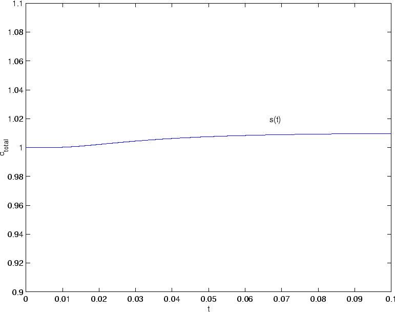
plot(t,s);
xlabel('t');
ylabel('c_{total}');
axis([0 0.1 0.9 1.1]);

Text version of this program

This program produces the following figures:

Figure 6: Numerical solution of the diffusion equation for different times with no-flux boundary conditions.

Figure 7: Verification that $s(t)$ is (approximately) constant.

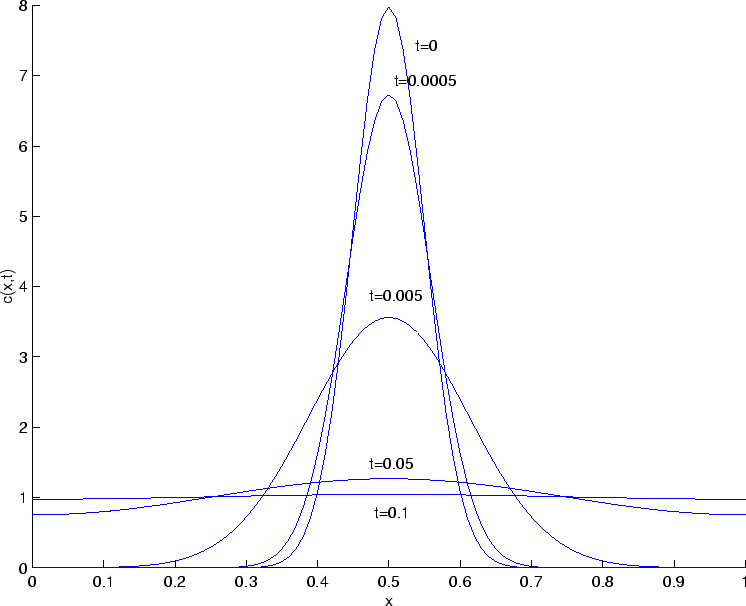We see that the solution eventually settles down to $c$ being uniform in $x$. Because of the normalization of our initial condition, this uniform state is given by $c = 1$. We also notice that $s(t)$ is not quite constant in time - this must be a result of numerical error (both in our finite difference scheme and our numerical calculation of integrals, etc). We could get a better result with different choices of $\delta x$ and $\delta t$, or by using a more sophisticated finite difference scheme.