Numerical Solution of the Diffusion Equation with Constant Concentration Boundary Conditions

The following Matlab code solves the diffusion equation according to the scheme given by (5) and for the boundary conditions $c(0,t) = c(1,t) = 0$. It also calculates the flux at the boundaries, and verifies that $s(t) + s_0(t) + s_1(t)$ is conserved.

numx = 101;   %number of grid points in x
numt = 2000;  %number of time steps to be iterated over 
dx = 1/(numx - 1);
dt = 0.00005;

x = 0:dx:1;   %vector of x values, to be used for plotting

C = zeros(numx,numt);   %initialize everything to zero

%specify initial conditions
t(1) = 0;      %t=0
C(1,1) = 0;    %C=0 at x=0
C(1,numx) = 0; %C=0 at x=1
mu = 0.5;
sigma = 0.05;
for i=2:numx-1
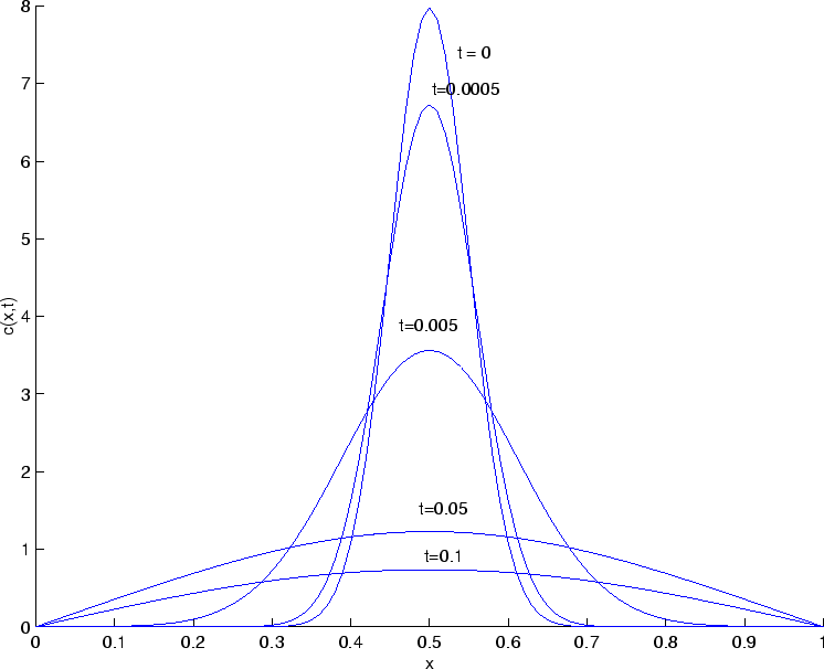
   C(i,1) = exp(-(x(i)-mu)^2/(2*sigma^2)) / sqrt(2*pi*sigma^2);
end

%iterate difference equation - note that C(1,j) and C(numx,j) always remain 0
for j=1:numt
   t(j+1) = t(j) + dt;
   for i=2:numx-1
      C(i,j+1) = C(i,j) + (dt/dx^2)*(C(i+1,j) - 2*C(i,j) + C(i-1,j)); 
   end
end

figure(1);
hold on;
plot(x,C(:,1));
plot(x,C(:,11));
plot(x,C(:,101));
plot(x,C(:,1001));
plot(x,C(:,2001));
xlabel('x');
ylabel('c(x,t)');

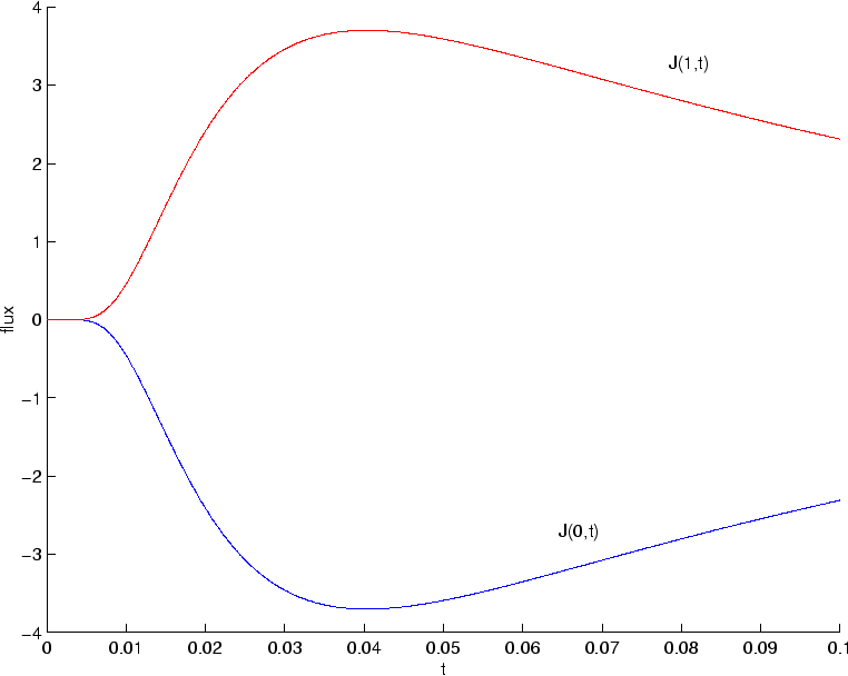
%calculate the flux at x=0 and x=1
for j=1:numt+1
   flux0(j) = -(C(2,j) - C(1,j))/dx;
   flux1(j) = -(C(numx,j)-C(numx-1,j))/dx;
end

figure(2);
hold on;
plot(t,flux0,'b');
plot(t,flux1,'r');
xlabel('t');
ylabel('flux');

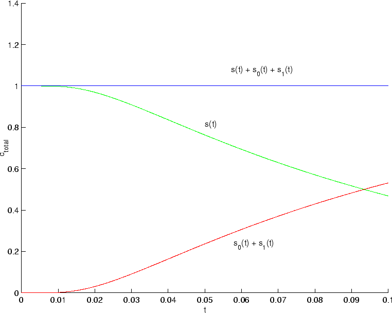
%calculate approximation to the integral of c from x=0 to x=1
for j=1:numt+1
   s(j) = sum(C(1:numx-1,j))*dx;
end

%calculate the amount of C that leaves through the boundaries due to flux
% s0 is the amount of C that leaves through x=0
% s1 is the amount of C that leaves through x=1
s0(1) = 0;
s1(1) = 0;
for j=1:numt
   s0(j+1) = s0(j) - flux0(j)*dt;
   s1(j+1) = s1(j) + flux1(j)*dt;
end

figure(3);
hold on;
plot(t,s,'g');
plot(t,s0+s1,'r');
plot(t,s+s0+s1,'b');

xlabel('t');
ylabel('c_{total}');

Text version of this program

This program produces the following figures:

Figure 3: Numerical solution of the diffusion equation for different times with $c(0,t) = c(1,t) = 0$.

Figure 4: The flux at $x=0$ (blue) and $x=1$ (red) as a function of time.

Figure 5: Verification that $s(t) + s_0(t) + s_1(t)$ is constant. Because of the normalization of our initial condition, this constant is equal to 1.

We see that for very short times, the concentration $c$ keeps its Gaussian shape; this is as expected from the diffusion equation in the absence of boundaries. However, eventually $c$ spreads out enough that the boundaries become important. Also, as expected from conservation of mass, we find that at all times $s(t) + s_0(t) + s_1(t)$ is constant.