Diffusion as a Smoother

Let's consider the diffusion equation with no-flux boundary conditions, and the initial condition

$$c(x,0) = 1 - 0.2 \cos(\pi x) + 0.1 \cos(2 \pi x) + 0.3 \cos(3 \pi x) + 0.1 \cos(8 \pi x) + 0.05 \cos(21 \pi x).$$

It is readily seen that this initial condition satisfies the no-flux boundary conditions, and also that

$$s(0) \equiv \int_0^1 c(x,0) dx = 1.$$

We expect that $s(t)=1$ for all times.

The following Matlab code solves the diffusion equation for no-flux boundary conditions and for this initial condition:

numx = 101;   %number of grid points in x
numt = 5000;  %number of time steps to be iterated
dx = 1/(numx - 1);
dt = 0.00005;

x = 0:dx:1;   %vector of x values, to be used for plotting

C = zeros(numx,numt);   %initialize everything to zero

%specify initial conditions
t(1) = 0;      %t=0
mu = 0.5;      
sigma = 0.05;
for i=1:numx
C(i,1) = 1 - 0.2*cos(pi*x(i)) + 0.1*cos(2*pi*x(i)) + 0.3*cos(3*pi*x(i)) + 0.1*cos(8*pi*x(i)) + 0.05*cos(21*pi*x(i));
end

%iterate difference equations
for j=1:numt
   t(j+1) = t(j) + dt;
   for i=2:numx-1
      C(i,j+1) = C(i,j) + (dt/dx^2)*(C(i+1,j) - 2*C(i,j) + C(i-1,j)); 
   end
   C(1,j+1) = C(2,j+1);          %C(1,j+1) found from no-flux condition
   C(numx,j+1) = C(numx-1,j+1);  %C(numx,j+1) found from no-flux condition
end

figure(1);
hold on;

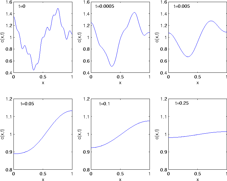
subplot(2,3,1);
plot(x,C(:,1));
axis([0 1 0.4 1.6]);
xlabel('x');
ylabel('c(x,t)');

subplot(2,3,2);
plot(x,C(:,11));
axis([0 1 0.4 1.6]);
xlabel('x');
ylabel('c(x,t)');

subplot(2,3,3);
plot(x,C(:,101));
axis([0 1 0.4 1.6]);
xlabel('x');
ylabel('c(x,t)');

subplot(2,3,4);
plot(x,C(:,1001));
axis([0 1 0.8 1.2]);
xlabel('x');
ylabel('c(x,t)');

subplot(2,3,5);
plot(x,C(:,2001));
axis([0 1 0.8 1.2]);
xlabel('x');
ylabel('c(x,t)');

subplot(2,3,6);
plot(x,C(:,5001));
axis([0 1 0.8 1.2]);
xlabel('x');
ylabel('c(x,t)');

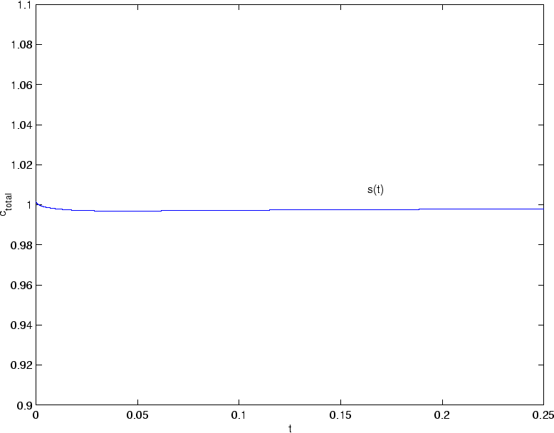
%calculate approximation to the integral of c from x=0 to x=1
for j=1:numt+1
   s(j) = sum(C(1:numx-1,j))*dx;
end

figure(2);
plot(t,s);
xlabel('t');
ylabel('c_{total}');
axis([0 0.25 0.9 1.1]);

Text version of this program

This program produces the following figures:

Figure 8: Numerical solution of the diffusion equation for different times.

Figure 9: Verification that $s(t) \approx 1$ for all $t$.

We see that the high wavenumber (short wavelength) components of $c$ get damped out very quickly - this is what we mean when we say that diffusion smooths out a solution. Notice that by $t=0.05$, the only components from the initial condition that are apparent are the ``constant'' component and the ``$\cos(\pi x)$'' component. The higher the wavenumber (i.e., the shorter the wavelength), the faster the mode is damped out.