Finally, using the program HHapprox.m, superimpose the trajectory corresponding to periodically firing action potentials onto the nullcline. This can be done, for example, with the following commands.
HHapprox
figure(2)
hold on;
plot(Y(400:500,1),Y(400:500,2),'g');
xlabel('V');
ylabel('n');
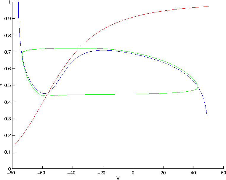
Here only the 400-450'th data points are plotted so that the transient does not appear. This gives the following figure:
Notice how the periodic orbit ``hugs'' the V-nullcline until reaching the
minimum or maximum, then abruptly ``jumps across'' from one branch
to another. Match up the pieces of this with the appropriate
events in the time series in Figure 4. Also, change the
input current to
![]() and use Matlab to plot the nullclines
and the periodic orbit found from integrating equations (2) and
(3). What happens for other values of
and use Matlab to plot the nullclines
and the periodic orbit found from integrating equations (2) and
(3). What happens for other values of ![]() ?
?