FitzHugh's Two-Dimensional Equations

With these simplifications, we are led to consider the following two-dimensional system of equations:

$$\frac{dV}{dt} = \{I - \bar{g}_{Na} [m_\infty(V)]^3 (0.8-n) (V-V_{Na}) - \bar{g}_K n^4 (V-V_K) - g_L (V-V_L)\}/C,$$ (2)

$$\frac{dn}{dt} = \alpha_n(V) (1-n) - \beta_n(V) n.$$ (3)

One could solve these using Euler integration as was used in Homework #1. However, here let's instead use the built-in Matlab function ode23, which uses second and third order Runge-Kutta algorithms. All other things being equal, higher order methods typically give more accurate approximate solutions. For more information on ode23 and other built-in functions to numerically solve ordinary differential equations, type ``help ode23'' at the Matlab prompt.

Download the following three files to integrate equations (2) and (3). First, the main program HHapprox.m:

global vna vk vl gna gk gl c I

vna=50; vk=-77;
vl=-54.4;
gna=120;
gk=36;
gl=.3;
c=1;
I=20;

[T,Y] = ode23('func_HHapprox',[0,100],[-65,.317]);

figure(1); subplot(2,1,1)
plot(T,Y(:,1));
xlabel('t');
ylabel('V');

subplot(2,1,2);
plot(T,Y(:,2));
xlabel('t');
ylabel('n');

Text version of this program

Next, the function func_HHapprox.m:

function dy = func_HHapprox(t,y)

global vna vk vl gna gk gl c I

v = y(1);
n = y(2);

dv = (I - gna*(m_inf(v))^3*(0.8-n)*(v-vna) - gk*n^4*(v-vk)-gl*(v-vl))/c;
dn = an(v)*(1-n)-bn(v)*n;

dy = [dv;dn];

Text version of this program

Next, the function am.m, which gives $\alpha_m(V)$:

function r= am(v)
r = .1*(v+40)/(1-exp(-(v+40)/10));

Text version of this program

Next, the function bm.m, which gives $\beta_m(V)$:

function r=bm(v)
r = 4*exp(-(v+65)/18);

Text version of this program

Next, the function an.n, which gives $\alpha_n(V)$:

function r=an(v)
r = .01*(v+55)/(1-exp(-(v+55)/10));

Text version of this program

Next, the function bn.m, which gives $\beta_n(V)$:

function r=bn(v)
r = .125*exp(-(v+65)/80);

Text version of this program

Finally, the function m_inf.m, which gives $m_\infty (V)$:

function r = m_inf(v)

global vna vk vl gna gk gl c I

r = am(v) / (am(v) + bm(v));

Text version of this program

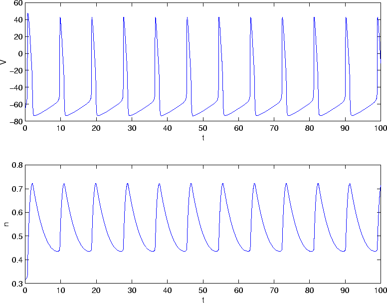
After downloading these programs, just type HHapprox at the Matlab prompt. This generates the following figure:

Figure 4: Timeseries for $V$ and $n$ found from solving equations (2) and (3).

Edit HHapprox.m to explore the dynamics for different values of the injected current $I$.