A Fast-Slow System

It can be shown numerically that when equations (2) and (3) exhibit periodically firing action potentials,

$$\left\vert \frac{dV}{dt} \right\vert \gg \left\vert \frac{dn}{dt} \right\vert.$$

Verify this. This implies that $V$ evolves much faster than $n$. We call $V$ a fast variable and $n$ a slow variable, and altogether equations (2) and (3) are a fast-slow system.

For fast-slow systems, a useful procedure for understanding the dynamics is to consider the nullclines. The V-nullcline is the set in $(V,n)$ space for which $\frac{dV}{dt}=0$, while the n-nullcline is the set in $(V,n)$ space for which $\frac{dn}{dt}=0$. It is messy to obtain analytical expressions for the nullclines of equations (2) and (3), but they can be computed numerically using the fzero command in Matlab which finds solutions $x$ of the equation $f(x)=0$. To do this, download the following three programs. First, nullclines.m:

global vna vk vl gna gk gl c I v

vna=50;
vk=-77;
vl=-54.4;
gna=120;
gk=36;
gl=.3;
c=1;
I = 20;

for i=1:130
v = -80 + i + 0.01;
vv(i) = v;
nullv(i) = fzero('rhsV',0.5);
nulln(i) = fzero('rhsn',0.5);
end

figure(2)
hold on;
plot(vv,nullv,'b');
plot(vv,nulln,'r');
axis([-80 60 0 1]);
xlabel('V'); ylabel('n');

Text version of this program

Next, rhsV.m, which is the righthand side of equation (2):

function r = rhsV(n)

global vna vk vl gna gk gl c I v

r = (I - gna*(m_inf(v))^3*(0.8-n)*(v-vna) - gk*n^4*(v-vk)-gl*(v-vl))/c;

Text version of this program

Finally, rhsn.m, which is the righthand side of equation (3):

function r = rhsn(n)

global vna vk vl gna gk gl c I v

r = an(v)*(1-n) - bn(v)*n;

Text version of this program

Note that in these programs, the membrane voltage (the Matlab variable ``v'') is treated as a global variable. This is because the functions that fzero uses need to be functions of a single, scalar variable. After downloading these programs, type ``nullclines'' at the Matlab prompt. You might get a few messages saying that Matlab was unable to find some zeros - this is OK. One obtains the following figure:

Figure 5: The nullclines for equations (2) and (3). The blue line is the V-nullcline, while the red line is the n-nullcline.

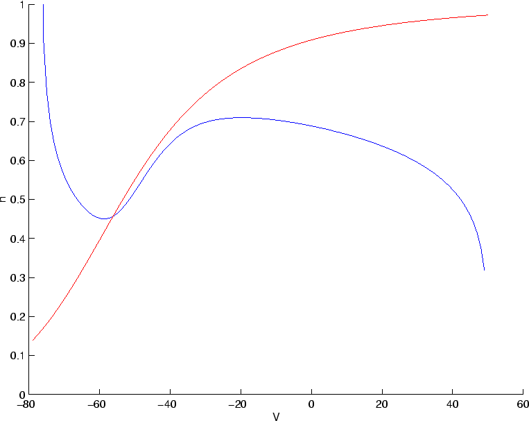Note that the point at which the nullclines intersect corresponds to a ``fixed point'' of equations (2) and (3). At this point, $\frac{dV}{dt}=\frac{dn}{dt}=0$.

Using the functions rhsV.m and rhsn.m, verify that

• $\frac{dV}{dt}>0$ below the V-nullcline
• $\frac{dV}{dt}<0$ above the V-nullcline
• $\frac{dn}{dt}>0$ below the n-nullcline
• $\frac{dn}{dt}<0$ above the n-nullcline