An SEIR model

We'll now consider the epidemic model from ``Seasonality and period-doubling bifurcations in an epidemic model'' by J.L. Aron and I.B. Schwartz, J. Theor. Biol. 110:665-679, 1984 in which the population consists of four groups:

• $S$ is the fraction of susceptible individuals (those able to contract the disease),
• $E$ is the fraction of exposed individuals (those who have been infected but are not yet infectious),
• $I$ is the fraction of infective individuals (those capable of transmitting the disease),
• $R$ is the fraction of recovered individuals (those who have become immune).

Note that the variables give the fraction of individuals - that is, we have normalized them so that

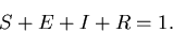$$S+E+I+R = 1.$$ (9)

Furthermore, suppose that

• There are equal birth and death rates $\mu$,
• $1/\alpha$ is the mean latent period for the disease,
• $1/\gamma$ is the mean infectious period,
• recovered individuals are permanently immune,
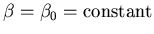
• the contact rate $\beta$ may be a function of time.

This leads us to consider the following model:

$$\frac{dS}{dt} = \mu - \beta(t) S I - \mu S$$ (10)

$$\frac{dE}{dt} = \beta(t) S I - (\mu + \alpha) E$$ (11)

$$\frac{dI}{dt} = \alpha E - (\mu + \gamma) I.$$ (12)

The variable $R$ is determined from the other variables according to equation (9). When $\beta = \beta_0 = {\rm constant}$, this is a three-dimensional autonomous system of ordinary differential equations, and is well understood. Defining

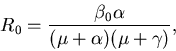$$R_0 = \frac{\beta_0 \alpha}{(\mu + \alpha) (\mu + \gamma)},$$ (13)

it can be shown that for $R_0>1$ the model has a fixed point with $I=0$ which is unstable, and a fixed point with $I>0$ which is stable, etc. See Aron and Schwartz for more detail and references.

If $\beta$ depends on time, we have a three-dimensional nonautonomous system, which can be converted to a four-dimensional autonomous system as was done above for the SIS model.