Let's explore what happens when the contact rate ![]() is a periodic
function of time. For example, for a childhood disease we might
imagine that
is a periodic
function of time. For example, for a childhood disease we might
imagine that ![]() is higher during the school year and lower during
the summer. Following the paper ``Asymptotic behavior in a deterministic
model'' by H.W. Hethcote, Bull. Math. Biol. 35:607-614, 1973,
let's take
is higher during the school year and lower during
the summer. Following the paper ``Asymptotic behavior in a deterministic
model'' by H.W. Hethcote, Bull. Math. Biol. 35:607-614, 1973,
let's take
| (4) |
| (5) |
| (6) | |||
| (7) |
global N alpha

gamma = 1;
N = 1;

options = odeset('MaxStep',0.01);
[T,Y] = ode45('func_SIS',[0 10],[0.2 0],options);

figure(1)
plot(T,Y(:,1));
xlabel('t');
ylabel('I');

for i=1:1000         %also plot a scaled version of beta
   tt(i) = 0.01*i;
   bb(i) = beta(tt(i));
end
hold on;
plot(tt,0.1*bb,'r');
Next, func_SIS.m:
function dy = func_SIS(t,y)

global N alpha

I = y(1);
tau = y(2);

dI = (beta(tau)*N - alpha)*I - beta(tau)*I^2;
dtau = 1;

dy = [dI;dtau];
Finally, beta.m:
function r = beta(t)

     r = 2 - 1.8*cos(5*t);
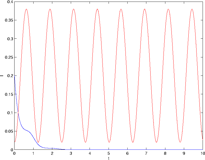
Figure 1 shows the numerical solution for this system with ![]() and
and ![]() in blue, and
in blue, and ![]() in red. It is seen that
in red. It is seen that ![]() decays to zero with a few wiggles in the transient.
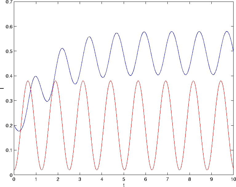
Figure 2 shows the numerical solution with
decays to zero with a few wiggles in the transient.
Figure 2 shows the numerical solution with ![]() and
and ![]() ,
again with
,
again with ![]() in red. Here
in red. Here ![]() settles into a periodically
oscillating state with period equal to the period of
settles into a periodically
oscillating state with period equal to the period of ![]() ; note that
the maximum of
; note that
the maximum of ![]() does not occur at the same time as the maximum of
does not occur at the same time as the maximum of ![]() .
.
To understand these results, Hethcote defines the average reproduction
number as
| (8) |