Following the paper by Aron and Schwartz, let's assume that
| (14) |
The following Matlab programs generate numerical solutions for this system. First SEIR.m:
global alpha beta0 beta1 gamma mu

mu = 0.02;
alpha = 35.84;
gamma = 100;
beta0 = 1800;
beta1 = 0.2;

options = odeset('MaxStep',0.01);
[T,Y] = ode45('func_SEIR',[0 50],[0.0658 0.0007 0.0002 0],options);

figure(1)
plot(T,-log(Y(:,3)));
xlabel('t');
ylabel('-ln(I)');

figure(2);
plot(-log(Y(:,1)),-log(Y(:,3)));
xlabel('-ln(S)');
ylabel('-ln(I)');
Text version of this program
function dy = func_SIS(t,y)

global alpha beta0 beta1 gamma mu

S = y(1);
E = y(2);
I = y(3);
tt = y(4);

dS = mu - beta_SEIR(tt)*S*I - mu*S;
dE = beta_SEIR(tt)*S*I - (mu + alpha)*E;
dI = alpha*E - (mu+gamma)*I;
ds = 1;

dy = [dS;dE;dI;ds];
Text version of this program
function r = beta_SEIR(t)

   global alpha beta0 beta1 gamma mu

   r = beta0*(1+beta1*cos(2*pi*t));
Text version of this program
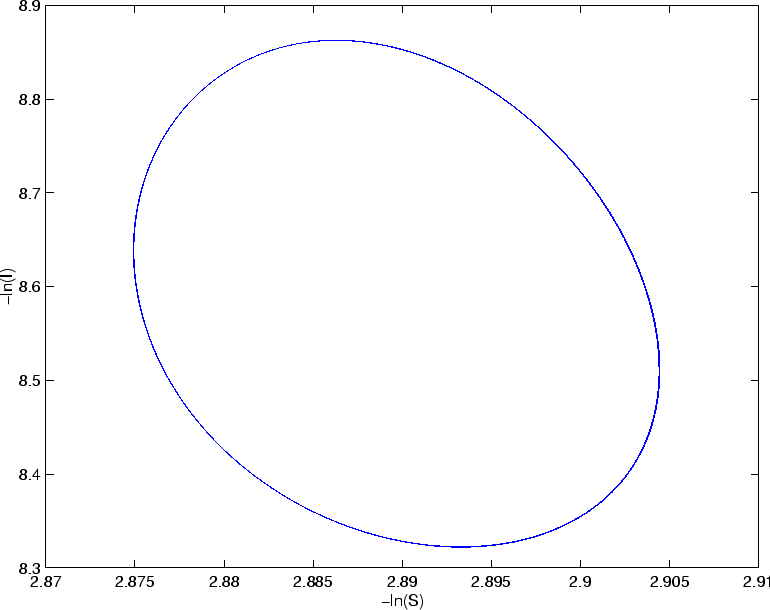
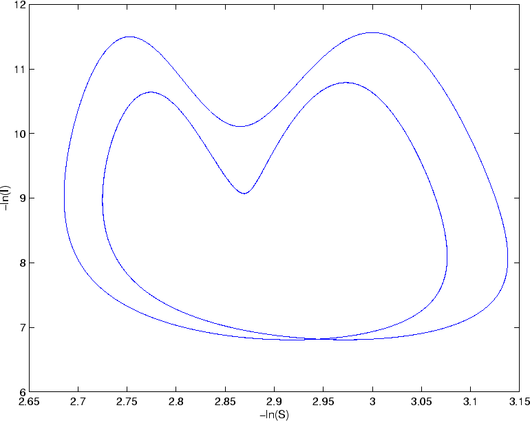
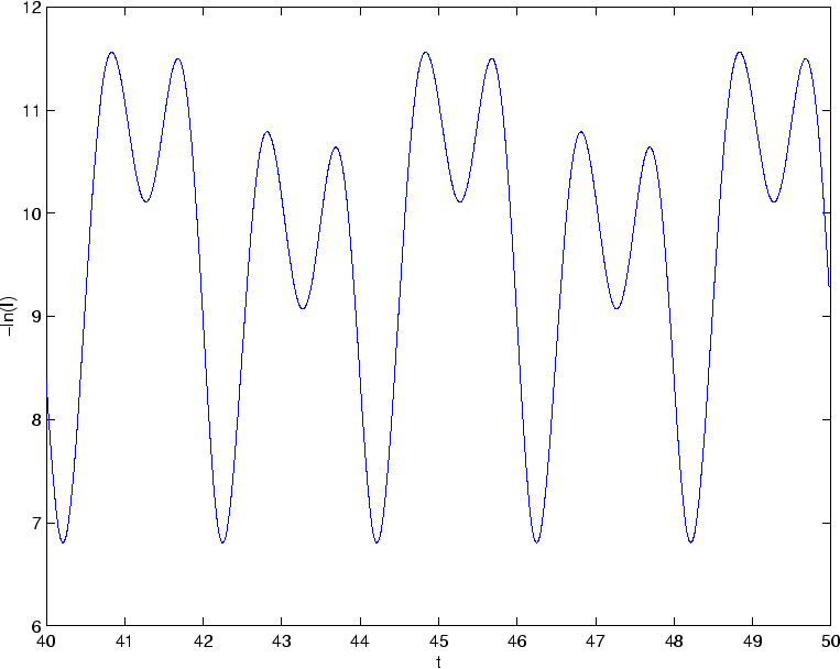
Playing around with the initial conditions and different values of
![]() , one finds the following solutions. Note that these figures
show the solution after integrating for a long time - therefore, they
give the asymptotically stable behavior. Also, it is most convenient
to plot minus the logarithm times the variables.
, one finds the following solutions. Note that these figures
show the solution after integrating for a long time - therefore, they
give the asymptotically stable behavior. Also, it is most convenient
to plot minus the logarithm times the variables.
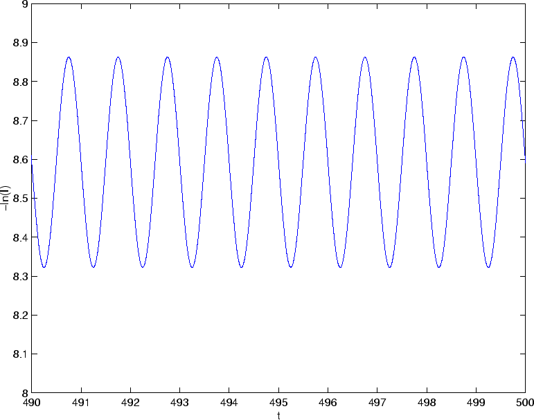
We see that at ![]() , the period of
, the period of ![]() is the same as the
period of
is the same as the
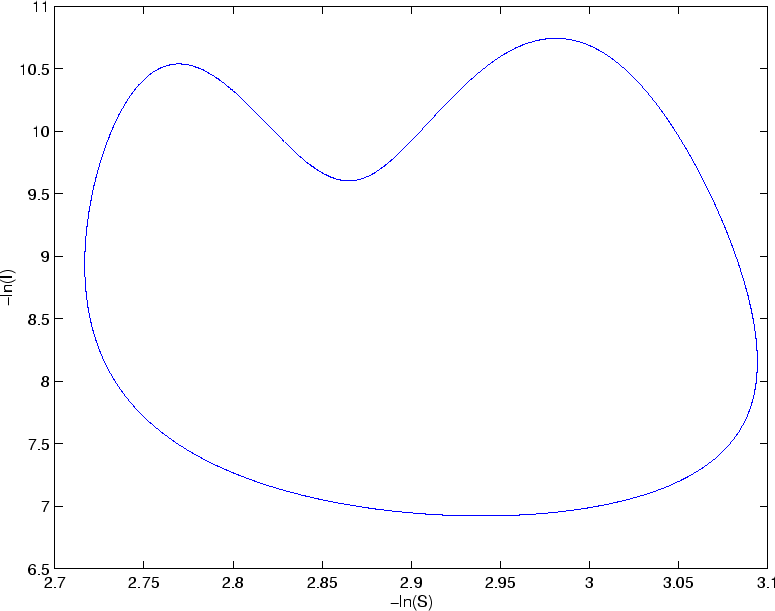
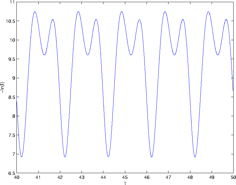
period of ![]() , namely 1. At
, namely 1. At ![]() , the period of
, the period of ![]() is twice the period of
is twice the period of ![]() . A period doubling bifurcation
has occurred between these values of
. A period doubling bifurcation
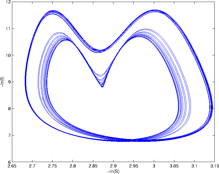
has occurred between these values of ![]() . Increasing
. Increasing ![]() to 0.26, another period doubling bifurcation occurs, and at
to 0.26, another period doubling bifurcation occurs, and at ![]() the period of
the period of ![]() is four times the period of
is four times the period of ![]() . Between
. Between
![]() and
and
![]() , an infinite number of such
period doubling bifurcations occur (this is called a period doubling
cascade). At
, an infinite number of such
period doubling bifurcations occur (this is called a period doubling
cascade). At
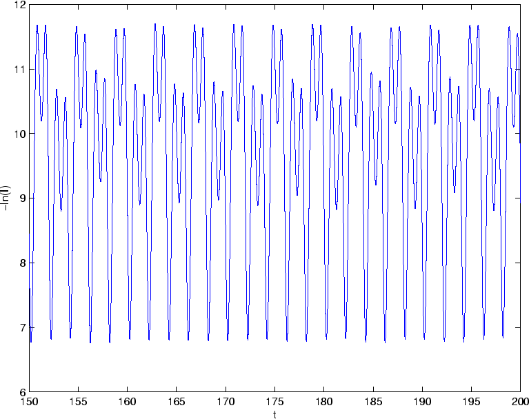
![]() the
solution is chaotic: it never exactly repeats itself!
the
solution is chaotic: it never exactly repeats itself!
A very important property of chaotic systems is that there is sensitive dependence on initial conditions, i.e., solutions which are close to each other at a given time will eventually diverge away from each other. Try integrating this model for two nearby initial conditions to see this property. In fact, you're encouraged to spend some time playing around with this model - you'll find a lot of surprises!