White noise ![]() is the formal derivative of a Wiener process
is the formal derivative of a Wiener process ![]() (this is a formal derivative because
(this is a formal derivative because ![]() has probability one of being
nondifferentiable). White noise has the properties
has probability one of being
nondifferentiable). White noise has the properties
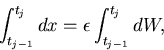
For example, consider the stochastic differential equation
| (2) |
 |
(3) |
| (4) |
In general, for the stochastic differential equation
| (5) |
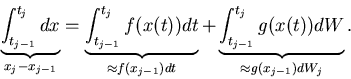
| (6) |
For example, suppose that we want to solve the formal equation
| (7) |
| (9) |
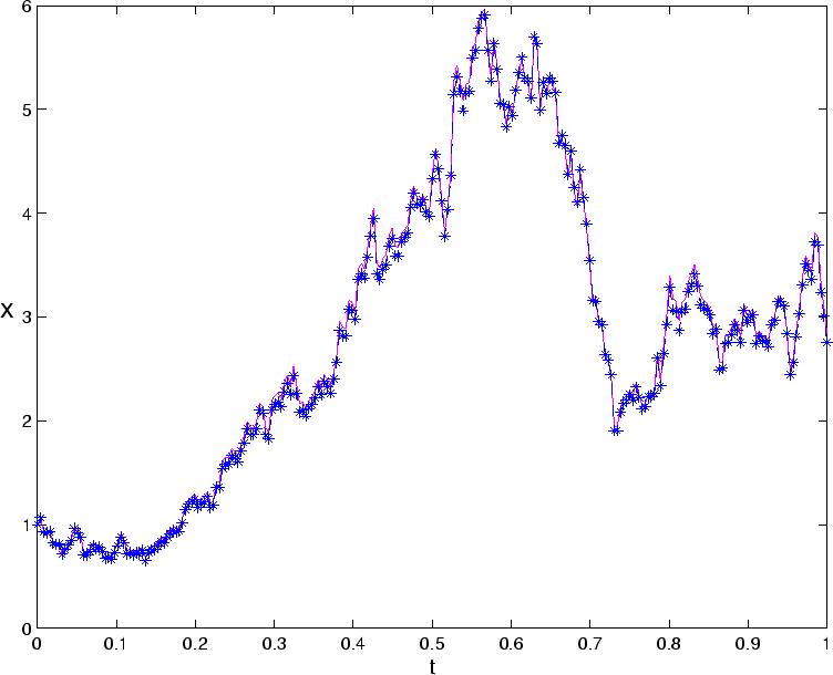
The following program em_simple.m is a slight modification of the program em.m from the article by Higham; it numerically solves equation (8) and compares to the exact solution.
%EM  Euler-Maruyama method on linear SDE
%
% SDE is  dX = lambda*X dt + mu*X dW,   X(0) = Xzero,
%      where lambda = 2, mu = 1 and Xzero = 1.
%
% Discretized Brownian path over [0,1] has dt = 2^(-8).
% Euler-Maruyama uses timestep dt.

randn('state',100)
lambda = 2                        % problem parameters
mu = 1;
Xzero = 1;
T = 1;
N = 2^8;
dt = 1/N;

dW = sqrt(dt)*randn(1,N);         % Brownian increments
W = cumsum(dW);                   % discretized Brownian path

Xtrue = Xzero*exp((lambda-0.5*mu^2)*([dt:dt:T])+mu*W);
plot([0:dt:T],[Xzero,Xtrue],'m-'), hold on

Xem = zeros(1,N);                 % preallocate for efficiency

Xem(1) = Xzero + dt*lambda*Xzero + mu*Xzero*dW(1);

for j=2:N
   Xem(j) = Xem(j-1) + dt*lambda*Xem(j-1) + mu*Xem(j-1)*dW(j);
end

plot([0:dt:T],[Xzero,Xem],'b--*'), hold off
xlabel('t','FontSize',12)
ylabel('x','FontSize',16,'Rotation',0,'HorizontalAlignment','right')

emerr = abs(Xem(end)-Xtrue(end))
 |