A Standard Wiener Process

A standard Wiener process (often called Brownian motion) on the interval $[0,T]$ is a random variable $W(t)$ that depends continuously on $t \in [0,T]$ and satisfies the following:

• $W(0) = 0$.
• For $0 \le s < t \le T$,
  
  $$W(t) - W(s) \sim \sqrt{t - s} N(0,1),$$
  
  
  where $N(0,1)$ is a normal distribution with zero mean and unit variance. Because the normal distribution is used, the process is oftened referred to as Gaussian.
• For $0 \le s < t < u < v \le T$, $W(t)-W(s)$ and $W(v)-W(u)$ are independent.

For use on a computer, we discretize the Wiener process with a timestep $dt$ as

$$dW \sim \sqrt{dt} N(0,1).$$

In Matlab, an element of the distribution $N(0,1)$ is obtained with the command ``randn''.

The article by Higham gives two equivalent Matlab programs to calculate a realization of a Wiener process. First bpath1.m:

%BPATH1  Brownian path simulation

randn('state',100)           % set the state of randn
T = 1; N = 500; dt = T/N;
dW = zeros(1,N);             % preallocate arrays ...
W = zeros(1,N);              % for efficiency

dW(1) = sqrt(dt)*randn;      % first approximation outside the loop ...
W(1) = dW(1);                % since W(0) = 0 is not allowed
for j = 2:N
   dW(j) = sqrt(dt)*randn;   % general increment
   W(j) = W(j-1) + dW(j); 
end

plot([0:dt:T],[0,W],'r-')    % plot W against t
xlabel('t','FontSize',16) 
ylabel('W(t)','FontSize',16,'Rotation',0)

Text version of this program

Next bpath2.m:

%BPATH2  Brownian path simulation: vectorized 

randn('state',100)          % set the state of randn
T = 1; N = 500; dt = T/N;

dW = sqrt(dt)*randn(1,N);   % increments
W = cumsum(dW);             % cumulative sum

plot([0:dt:T],[0,W],'r-')   % plot W against t
xlabel('t','FontSize',16)
ylabel('W(t)','FontSize',16,'Rotation',0)

Text version of this program

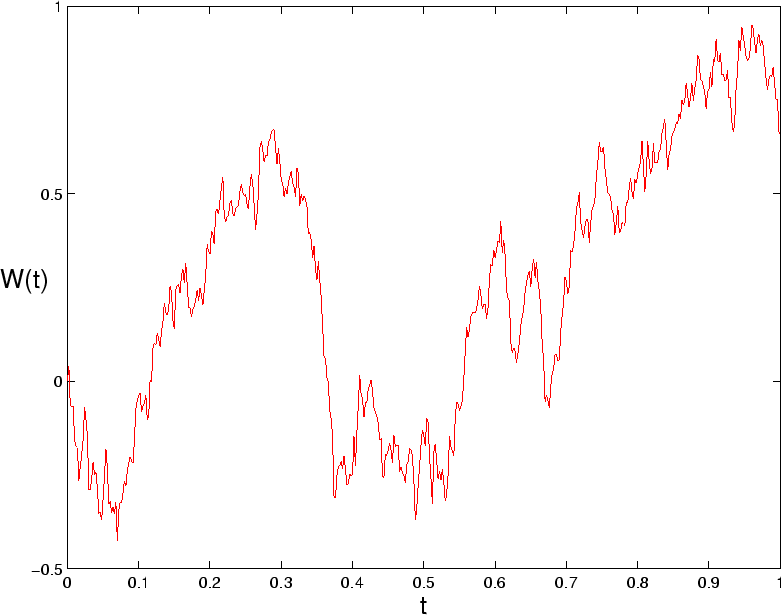
These programs produce Figure 1.

Figure 1: A realization of a Wiener process.