Bursting Behavior

Figure 6 sketches how the bursting behavior of equations (3-5) is related to the bifurcation analysis of equations (6,7).

Figure 6: Sketch of how the bursting behavior is related to the bifurcation analysis of equations (6,7).

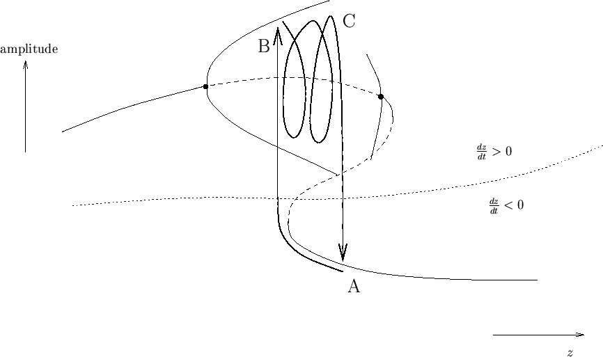Suppose that we start at point A. We are on a fixed point of equations (6,7), which corresponds to the rest state of the neuron. Now, $z$ will slowly decrease and we follow this branch of fixed points until we reach the saddlenode bifurcation. Here the system makes a jump to point B, i.e., to the stable periodic orbit, which corresponds to the active state. Now, $z$ will slowly increase with the neuron actively firing until we reach the homoclinic bifurcation at C. Here the periodic orbit ceases to exist and the system makes a jump back to point A, i.e, to the fixed point. This behavior repeats, giving a sequence of bursts. Note that as the homoclinic bifurcation is approached, the period of the periodic orbits increases - this is an example of adaptation as described in the lectures.

Verify from the time series in Figure 4 that the variables are behaving as described above, and that the jumps between the rest and active states occur near the values of $z$ at which the appropriate bifurcations of equations (6,7) occur.

It is interesting to modify the Matlab programs to see how the bursting behavior is affected. For example, what happens if $r$ is decreased? What happens for larger $I$, say $I=4$, or smaller $I$, say $I=0.4$?