Treating $z$ as Fixed in the Simple Model

From our numerical simulations, we see that the variable $z$ does not vary quickly during either the rest or the active states. Mathematically, this is due to the fact that $r$ was taken to be very small. This leads us to consider the two-dimensional system of equations where $z$ is treated as a constant:

$$\frac{dx}{dt} = y - x^3 + 3 x^2 + I - z$$ (6)

$$\frac{dy}{dt} = 1 - 5 x^2 - y$$ (7)

Figure 5 is a sketch of the results of a numerical bifurcation analysis for these equations, where we take $I=2$ and $z$ is treated as a bifurcation parameter.

Figure 5: Bifurcation diagram for equations (6,7) with $I=2$ and $z$ treated as a bifurcation parameter. Solid lines indicate stable solutions, while dashed lines indicate unstable solutions. Fixed points are labelled $f.p.$, and periodic orbits are labelled $p.o.$. The dotted line shows where $dz/dt=0$ from equation (5).

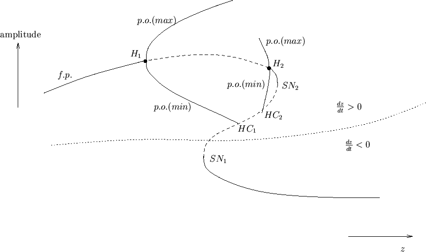The bifurcations for $I=2$ are as follows:

• $H_1$: Hopf bifurcation at $z=-9.593136$
• $H_2$: Hopf bifurcation at $z=2.926472$
• $SN_1$: saddlenode bifurcation of fixed points at $z = 1.814815$
• $SN_2$: saddlenode bifurcation of fixed points at $z = 3$
• $HC_1$: homoclinic bifurcation at $z = 2.085601$
• $HC_2$: homoclinic bifurcation at $z=2.926472$