Euler's Method

Consider the initial value problem

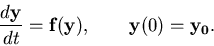$$\frac{d {\bf y}}{d t} = {\bf f}({\bf y}), \qquad {\bf y}(0) = {\bf y_0}.$$ (1)

Suppose we write the Taylor exansion of the solution:

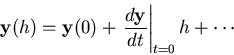$${\bf y}(h) = {\bf y}(0) + \left.\frac{d {\bf y}}{d t} \right\vert _{t=0} h + \cdots$$ (2)

Truncating and using (1), we obtain the formula for Euler's method for the numerical solution of differential equations:

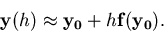$${\bf y}(h) \approx {\bf y_0} + h {\bf f}({\bf y_0}).$$ (3)

Of course, there is nothing special about $t=0$, so, letting ${\bf y}_n \equiv {\bf y}(t_n)$, $t_n \equiv n h$, we obtain

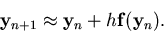$${\bf y}_{n+1} \approx {\bf y}_n + h {\bf f}({\bf y}_n).$$ (4)

By iterating, we find an approximation to the solution $y(t)$ of (1). Here $h$ is known as the stepsize.