Adaptive Networks & Heteroclinic Dynamics

We show some examples below of adaptivity in an N cell network of coupled odd logistic maps $f(x) = a x (1 - x^2)$. (We should emphasize that what we show is but a small sample of some of the remarkable dynamics that can occur!) The odd logistic map is scaled to give a self-map of [0,1], computations are done mod 1 and the coefficient $a \in [-3,3]$. We consider cases where cells are identical and approximately identical. Coupling strengths (weights) are limited to lie in the range [0, 2.00] and then multiplied by c/number of cells where c > 0. Initial conditions are chosen randomly in the interval [0.1,0.8]; initial weights are chosen randomly and lie in [0.3,0.8]. Coupling is either all-to-all or with a given sparseness which ranges zero (no coupling) to 1 (all-to-all). When we rescale we keep $c \times \text{sparseness}$ constant. We show dynamics of the cells and also weight averages for each node. The weight average measures the average over all inputs to a given node. It is also possible to show the evolution of the time averages of weights (we don't show that here). Currently we can simulate between $N=4$ and $N=10,000$ cells. We use various types of adaption (a total of 12 currently) including 'global' schemes based on work of Ito-Kaneko, 2002, 2003 and what we term 'fake STDP'. For the images we show here, we strengthen weights (both ways) between cells i and j if states of i and j are close and weaken if they are not close (we call an asymmetric directed version of this rule fake STDP). Typically we use adaptation of the form $$w^{n+1}_{ij} = (1 + C (1 - D|x_i - x_j|))w^n_{ij},$$ where $C,D > 0$ and $x_i$ denotes state of cell i at time n (or n+1), and $w^n_{ij}$ is the weight at time n for the connection from cell j to cell i. We note that the size of this computation per iteration grows like $aN^2$, where a is independent of N (a is at least 10). This is a significant computation for a 'desktop' computer when N = 10,000 and we do say 12,000 iterations (order $10^{13}$ computations). Almost all the computations we show here were done in extended precision (long double) and are sensitive to small quantities of the order $10^{-4900}$. This is necessary to pick up some of the heteroclinic phenomena over extended time periods. The software is based on prism, used in the past for computation of symmetric attractors and patterns, and is partly parallelized (threaded). 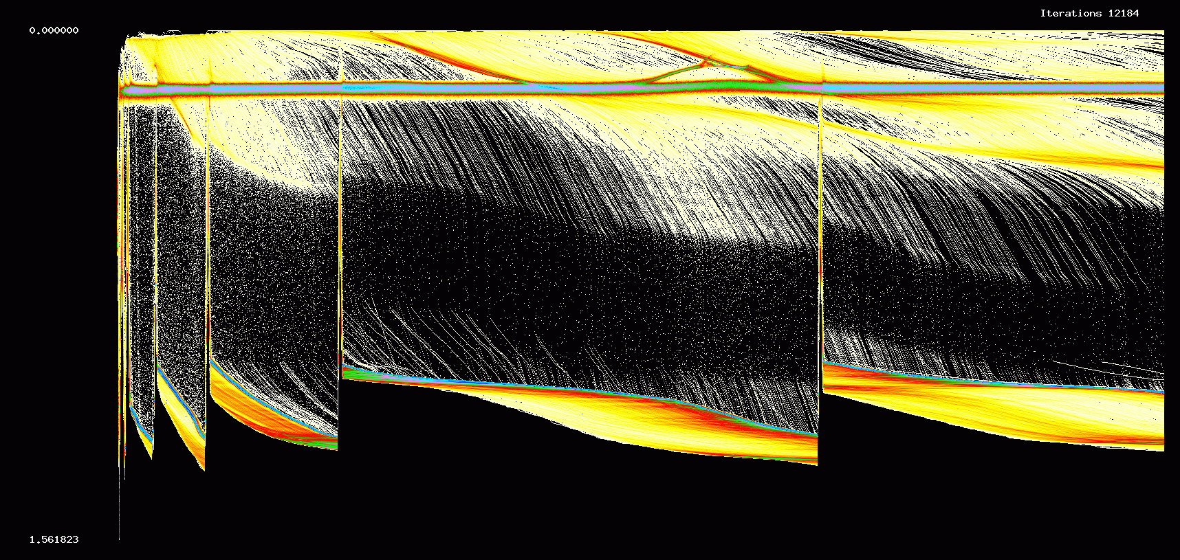In Figures 1 and 2 we assume 200 cells, 12184 iterations. We assume identical odd logistic maps with a = 2.31. Figure 1 shows dynamics, Figure 2 the evolution of averages of in weights from each cell. Figure 1. Dynamics, a = 2.31 Figure 2. Evolution of average in-weights at nodes. We remark the complexity of the initial transient which shows characteristic features of a heteroclinic cycle (between chaotic sets). However, the heteroclinic phenomena is closely tied to the adaptivity. Run for a sufficiently long time, the network will reach a `steady state'. See Figure 3 below which shows dynamics over an interval of 121,840 iterations, starting at 365,520 iterations. Further iteration leaves the picture unchanged. Figure 3. Long term dynamics. 121,840 iterations, starting at 365,520. The transient and long term structure appears relatively independent of the number of cells. 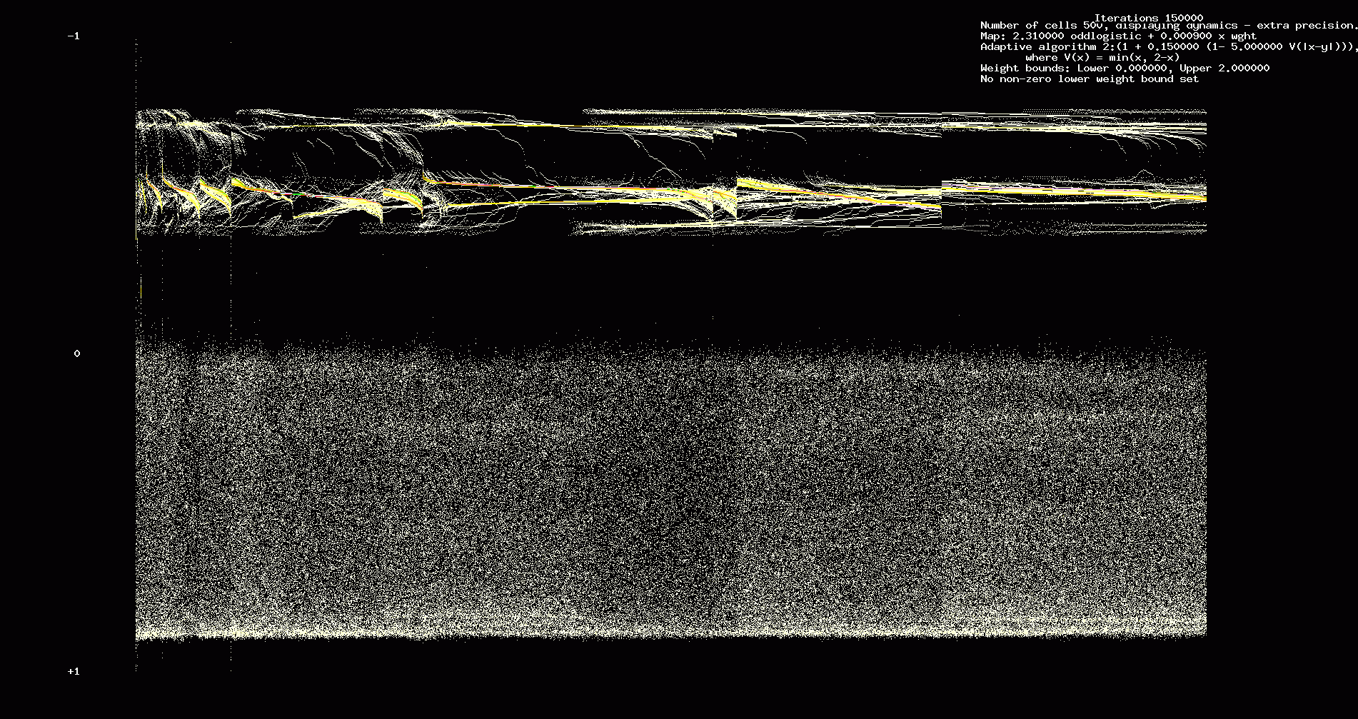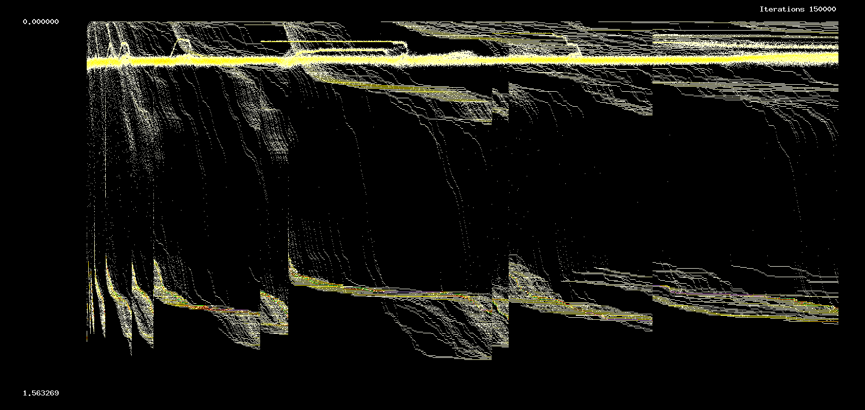In the next two figures we show the first 150,000 iterations of a network with 500 cells. Parameters are similar to those of the 200 cell network. Figure 4. Dynamics 500 cell network: 150,000 iterations Figure 5. 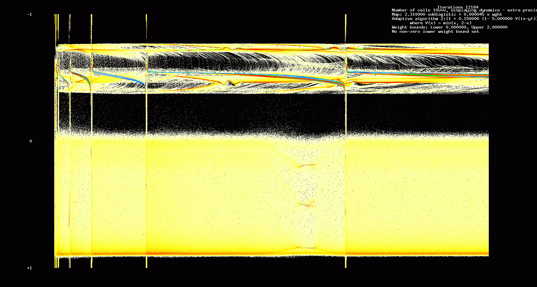Weight averages for 500 cell network: 150,000 iterations In the next two figures we show the first 12,184 iterations of a 10000 cell network with the same parameters used in Figures 1,2. Figure 6. Dynamic transients: 10000 cell network, 12,184 iterations Figure 7. 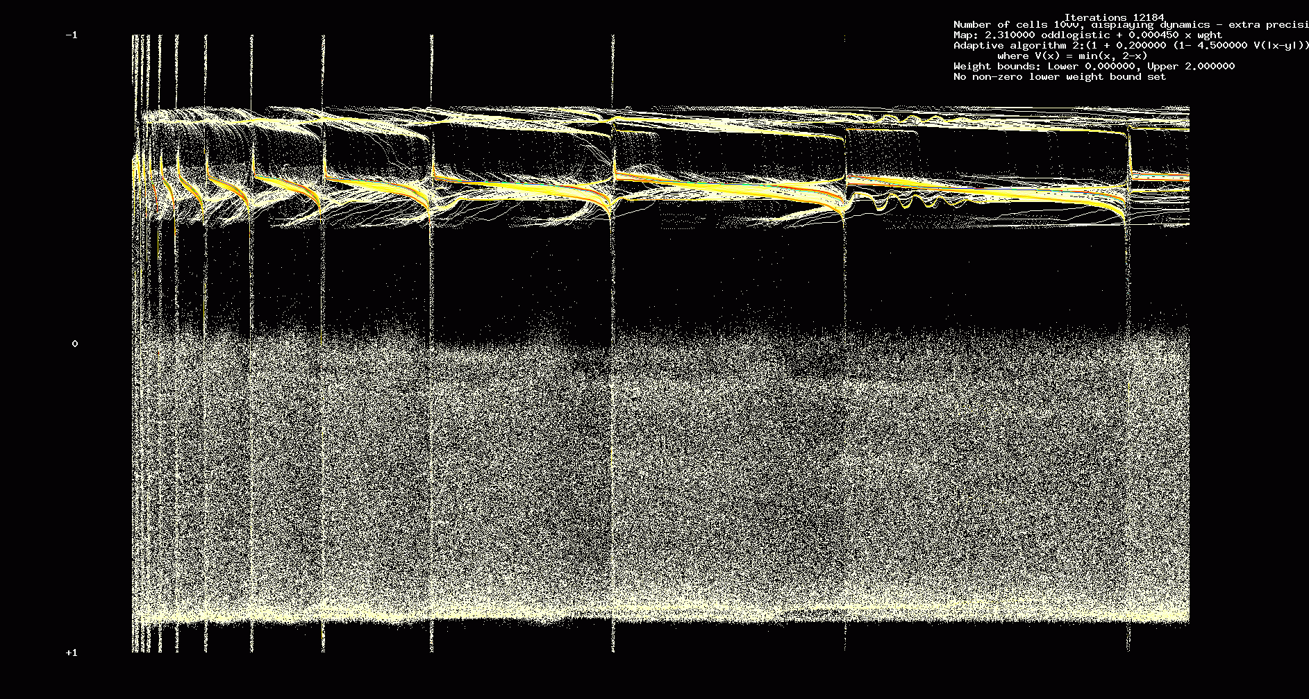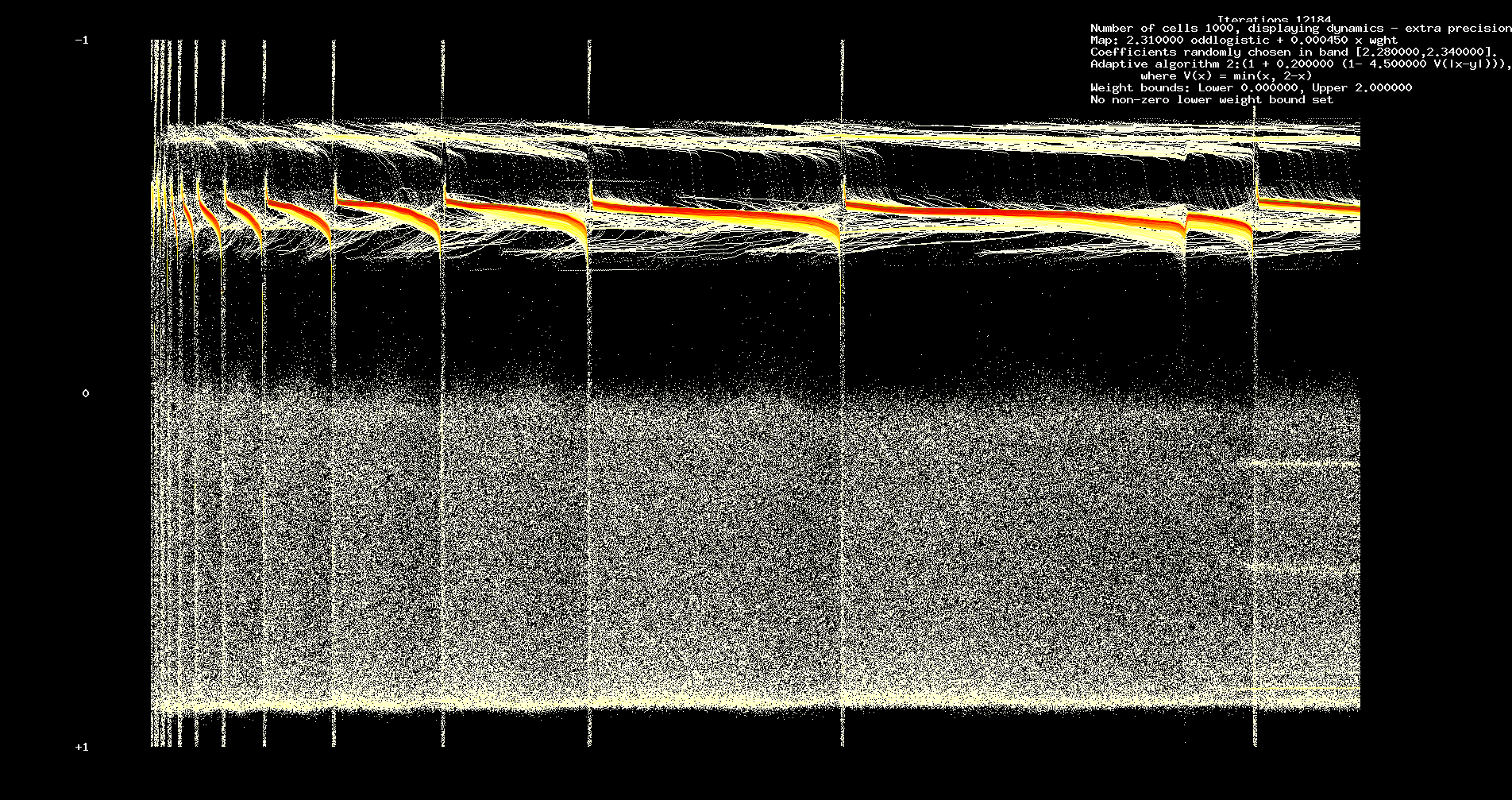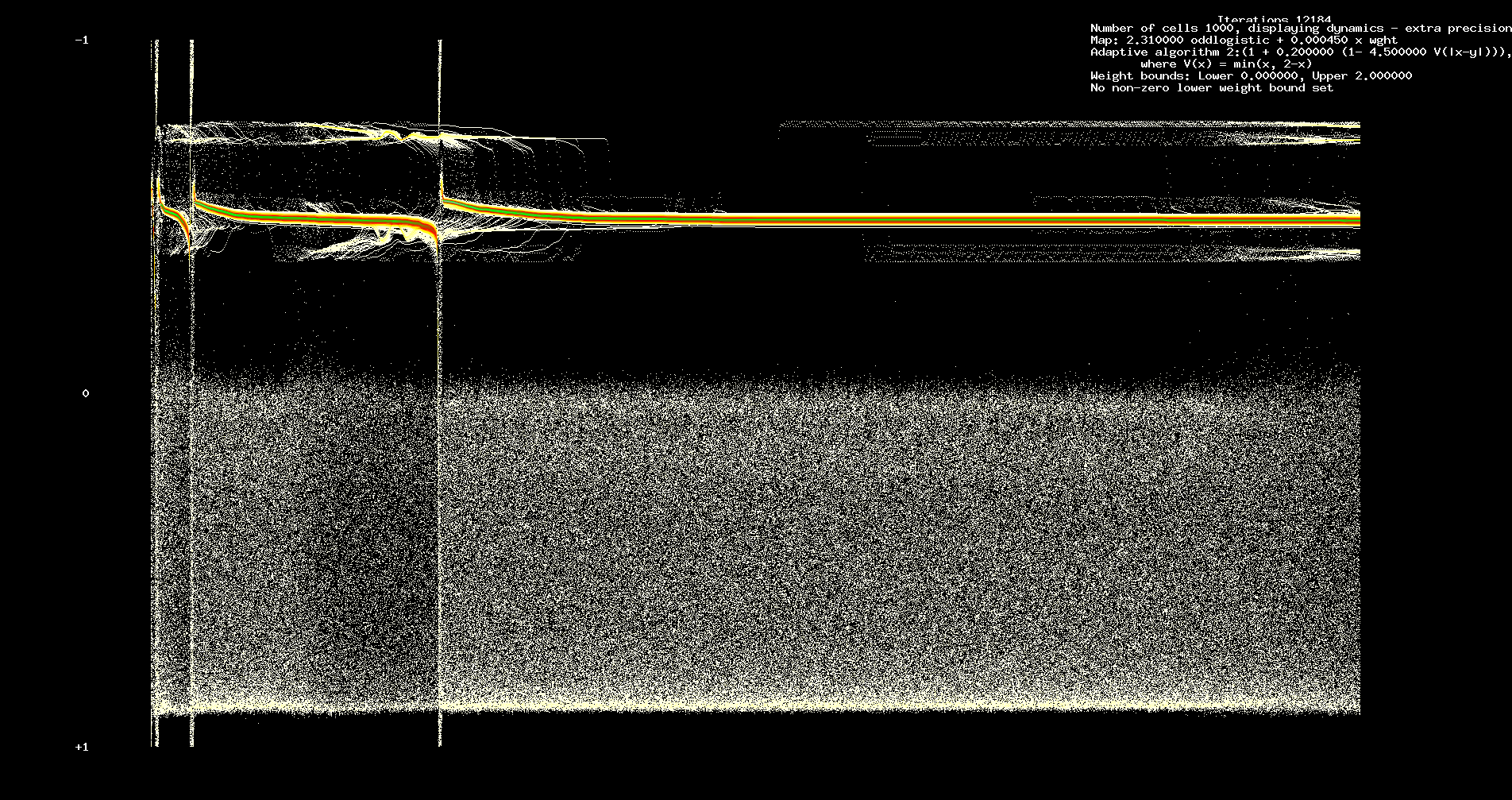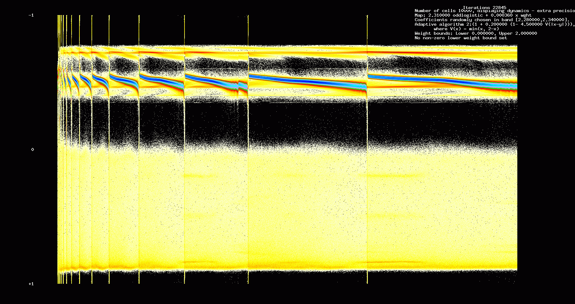Evolution of weights: 10000 cell network, 12,184 iterations In the next set of figures, which are all for a 1000 cell network, we (a) break the identical cell structure and allow for uniform distribution of the coefficients of the odd logistic map in a small interval, (b) show the effects of decreasing the sparseness of the coupling. First we show the results when we assume identical odd logistic maps and all to coupling. Figure 8. Dynamics, 1000 identical cells, sparseness = 1, 12,184 iterations Next we show dynamics when coefficients of the logistic maps are uniformly distributed in the interval [2.28,2.34]. Figure 9. 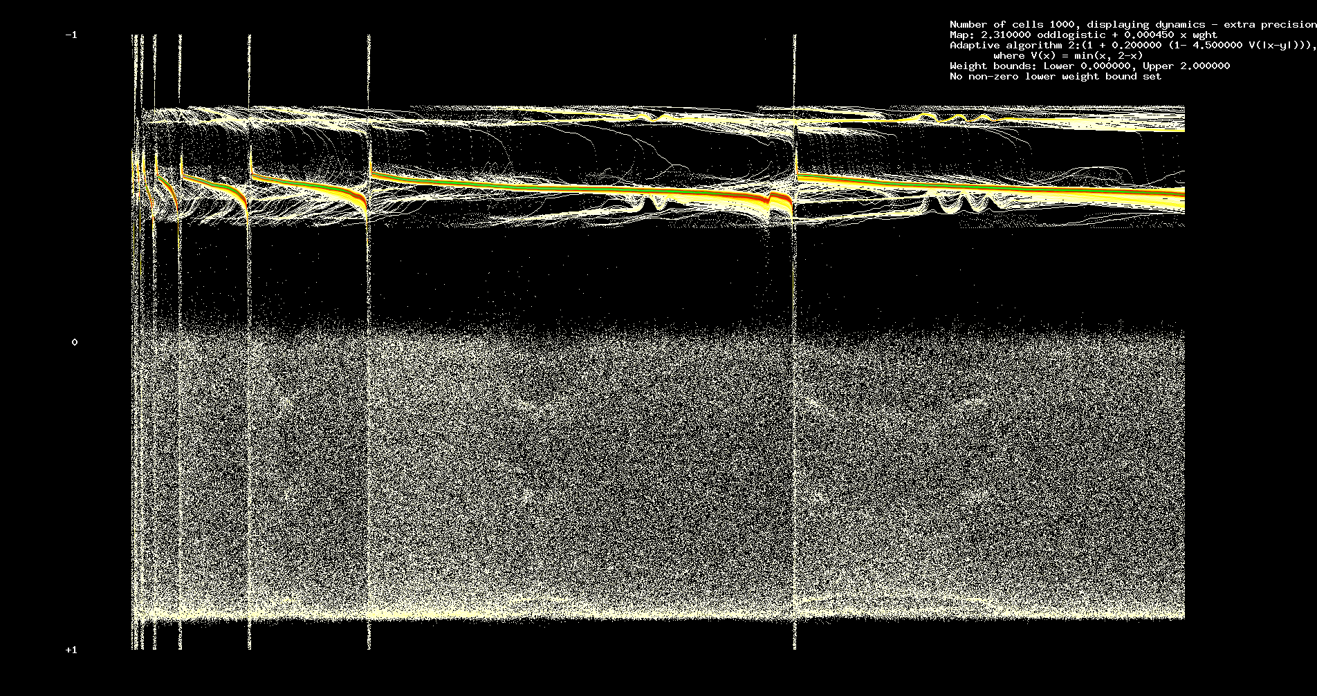Dynamics, 1000 non-identical cells, sparseness = 1, 12,184 iterations In Figure 10, we have identical cells but the sparseness of coupling is 0.9. As can be seen the transient behaviour is relatively unaffected. Figure 10. Dynamics, 1000 identical cells, sparseness = 0.9, 12,184 iterations In Figure 11, we have identical cells and the sparseness of coupling is 0.8. As can be seen the transient behaviour is now changed. Figure 11. 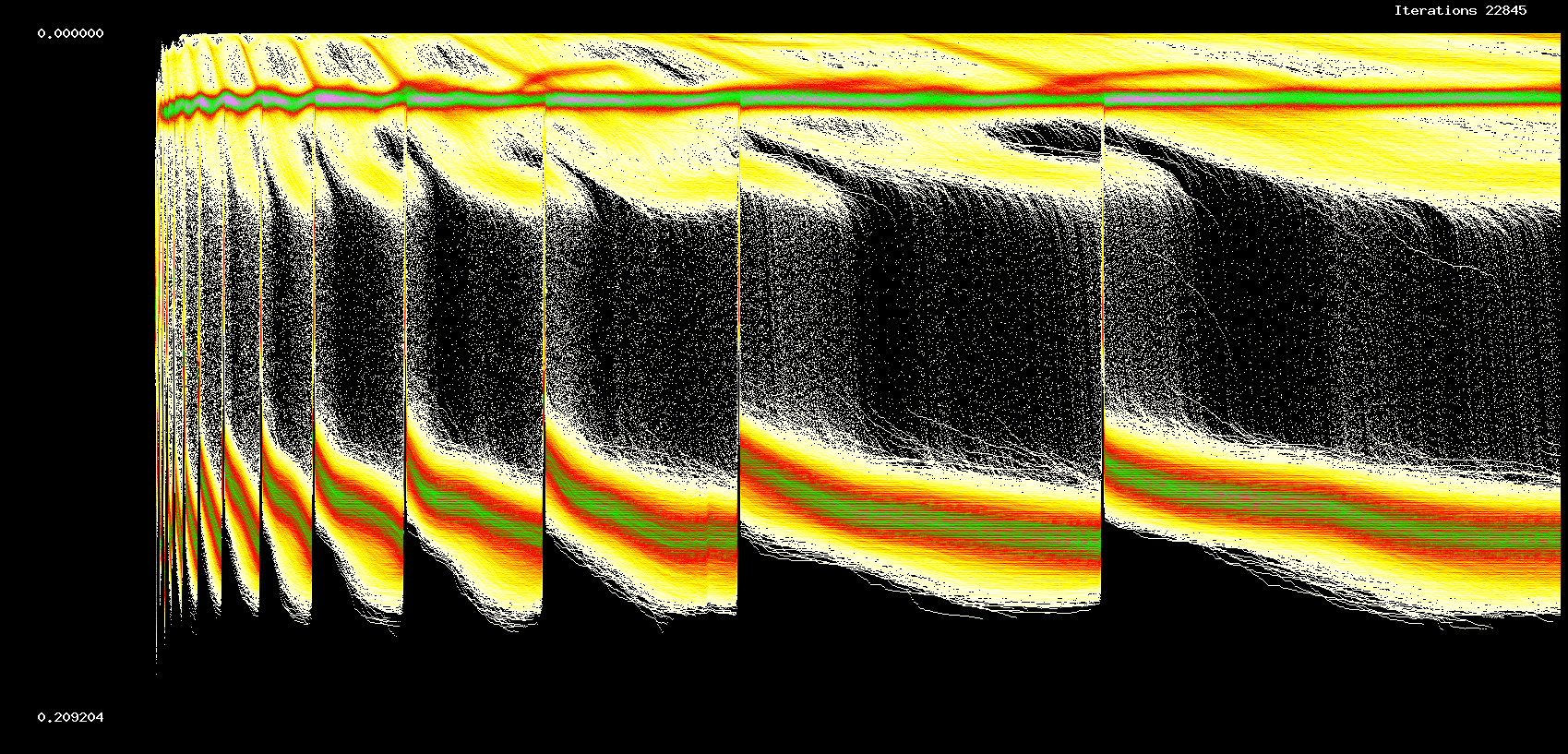Dynamics, 1000 identical cells, sparseness = 0.8, 12,184 iterations However, more can be said about this example: under a natural rescaling, heteroclinic behaviour persists even for low sparseness and non-identical cells. In the next two figures we show dynamics and weight evolution for a 10000 cell network, sparseness 0.125 and coefficients of the odd logistic map randomly distributed in an interval [2.31-0.03,2.31+0.03]. Fig. 12. Dynamics, 10000 non-identical cells, sparseness = 0.125, 22,845 iterations Fig. 13. 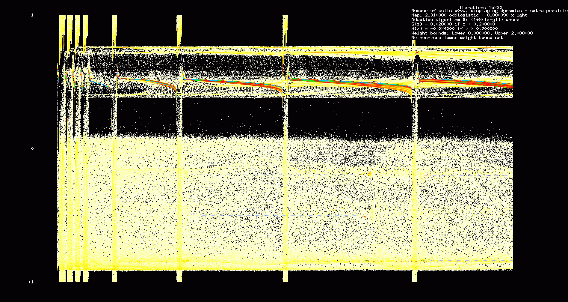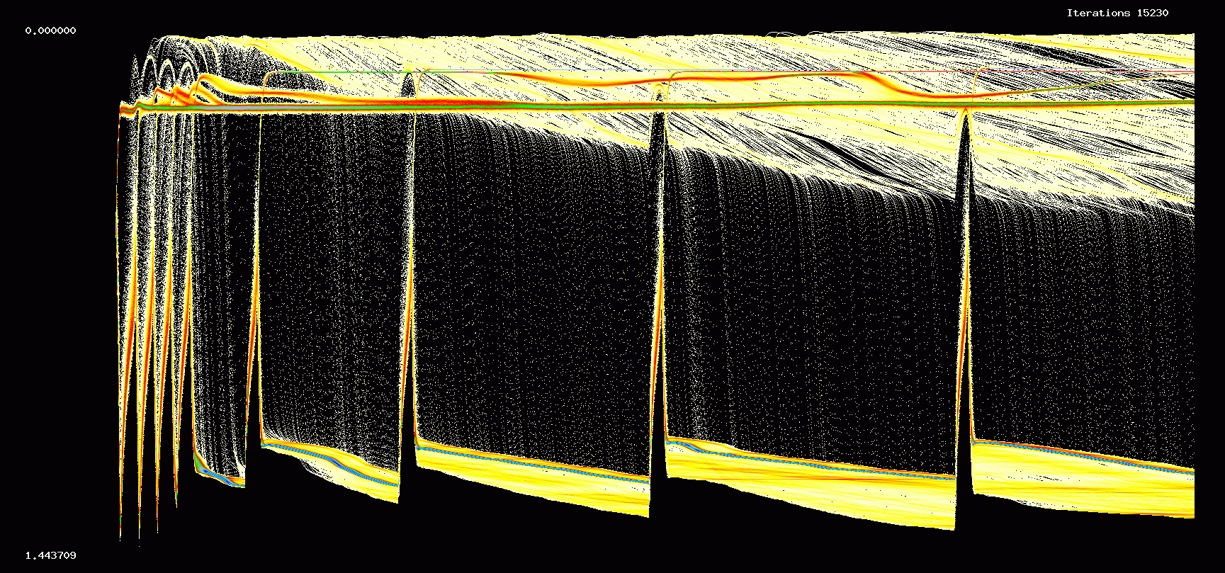Node Weights, 10000 non-identical cells, sparseness = 0.125, 22,845 iterations In the next two figures, we show network adaptation using a different adaptive scheme (bang-bang type control). We assume that weights evolve according to $$w_{ij}^{n+1} = (1 + W(\theta_i,\theta_j))w_{ij}^n,$$ where $W(x,y) = a$, if $|x-y| < \alpha$, $W(x,y) = -b$ if $|x-y| \geq \alpha$, where $0 < a < b < 1$ and typically $a,b$ are small. We continue to assume that weights are constrained to lie in [0,2]. Fig. 14. Dynamics. 5000 identical cells, 'bang-bang' type adaptation, 15,230 iterations. Fig. 15. Weights. 5000 identical cells, 'bang-bang' type adaptation, 15,230 iterations. 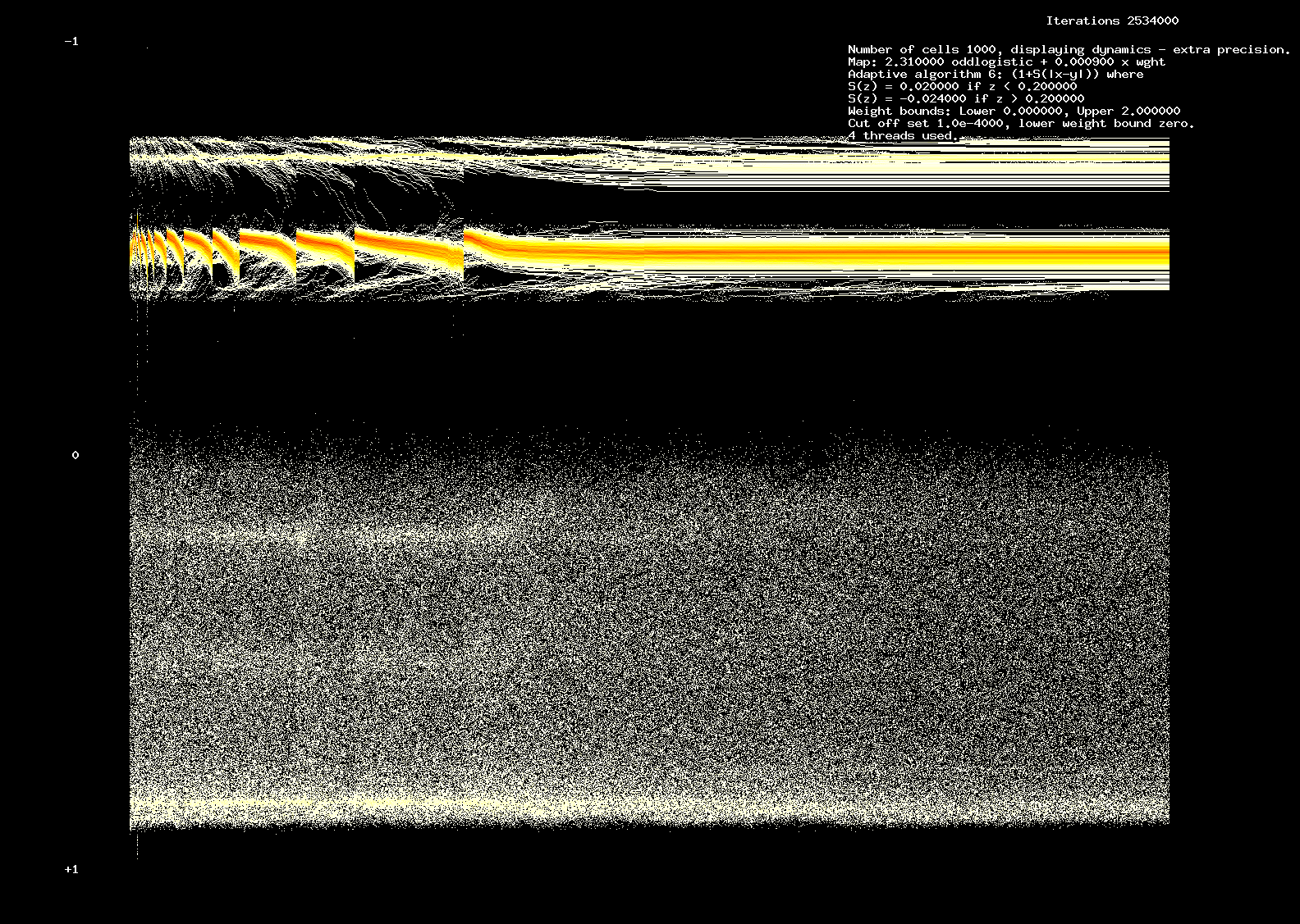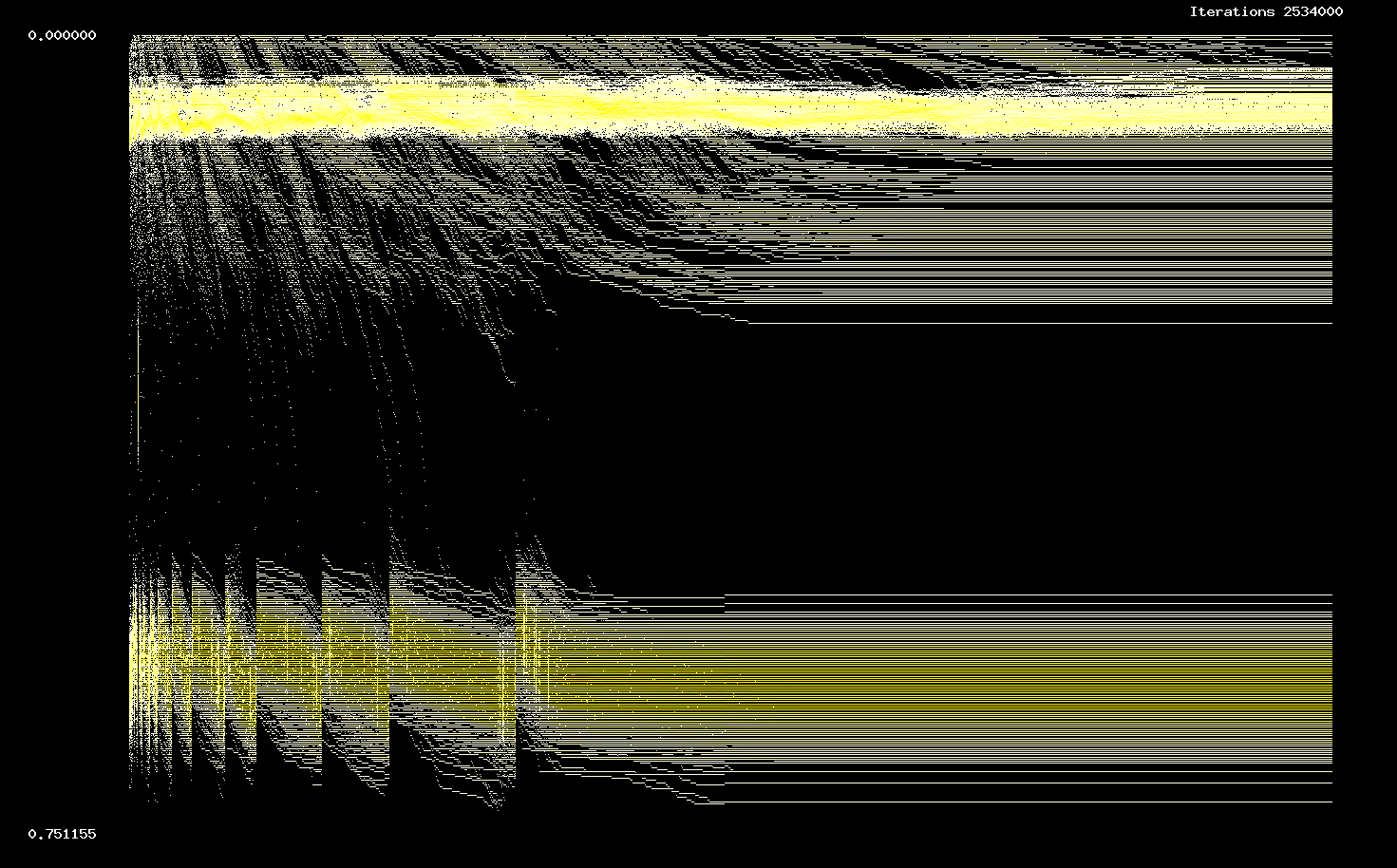Next we show a simulation of a 1000 cell network over 2.534 million times steps (points are plotted every 2000 time steps). This is quite a big computation but the evolution is similar to what we have shown before: eventually the system settles down to a steady state. 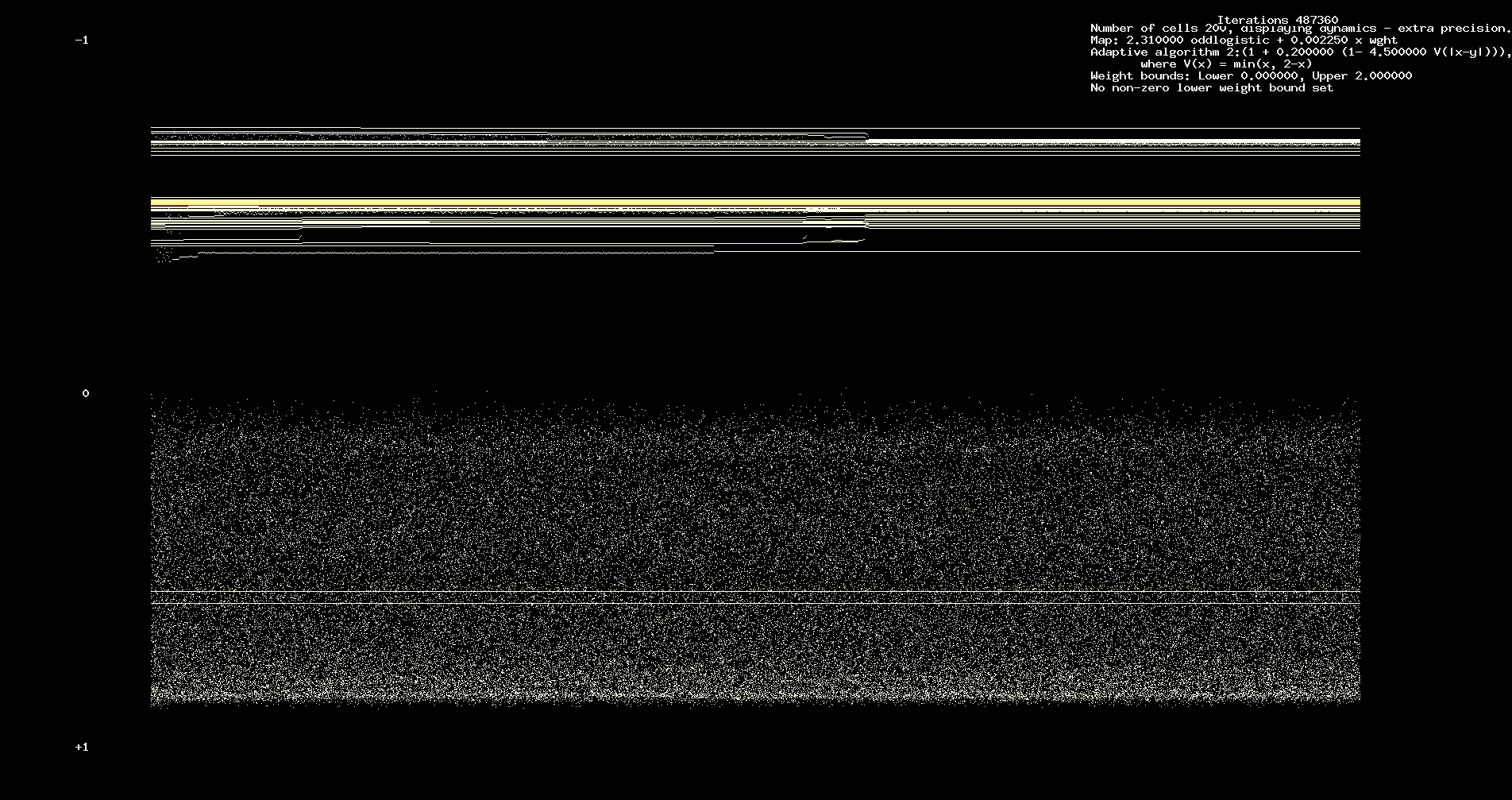We use the same adaptive algorithm as in Figure 14 and assume sparseness of coupling is 0.5. Other parameters are the same as those used for the network of Figure 14. In particular, we assume a=2.31. Figure 16. Dynamics, 1000 cells, 2.534 million iterations Figure 17. Evolution of weights, summed over each node. Synchronous and asynchronous computation and SLOGALS A digital computer computes synchronously: computations are timed to a clock. If the computation is threaded (or parallelized), then pieces of the computation are done synchronously but the synchronous blocks are handled asynchonously. Globally Asynchronous Locally Synchronous (GALS for short). A classic problem with threaded programming is getting global synchronization of the threads correct. For example, if thread A is using computations of thread B, we need to be sure that thread B has finished the needed computations before thread A uses them. Harder than it looks and the resulting code can be hard to debug. In general, getting the asynchronous logic correct is much more costly than the synchronous logic. 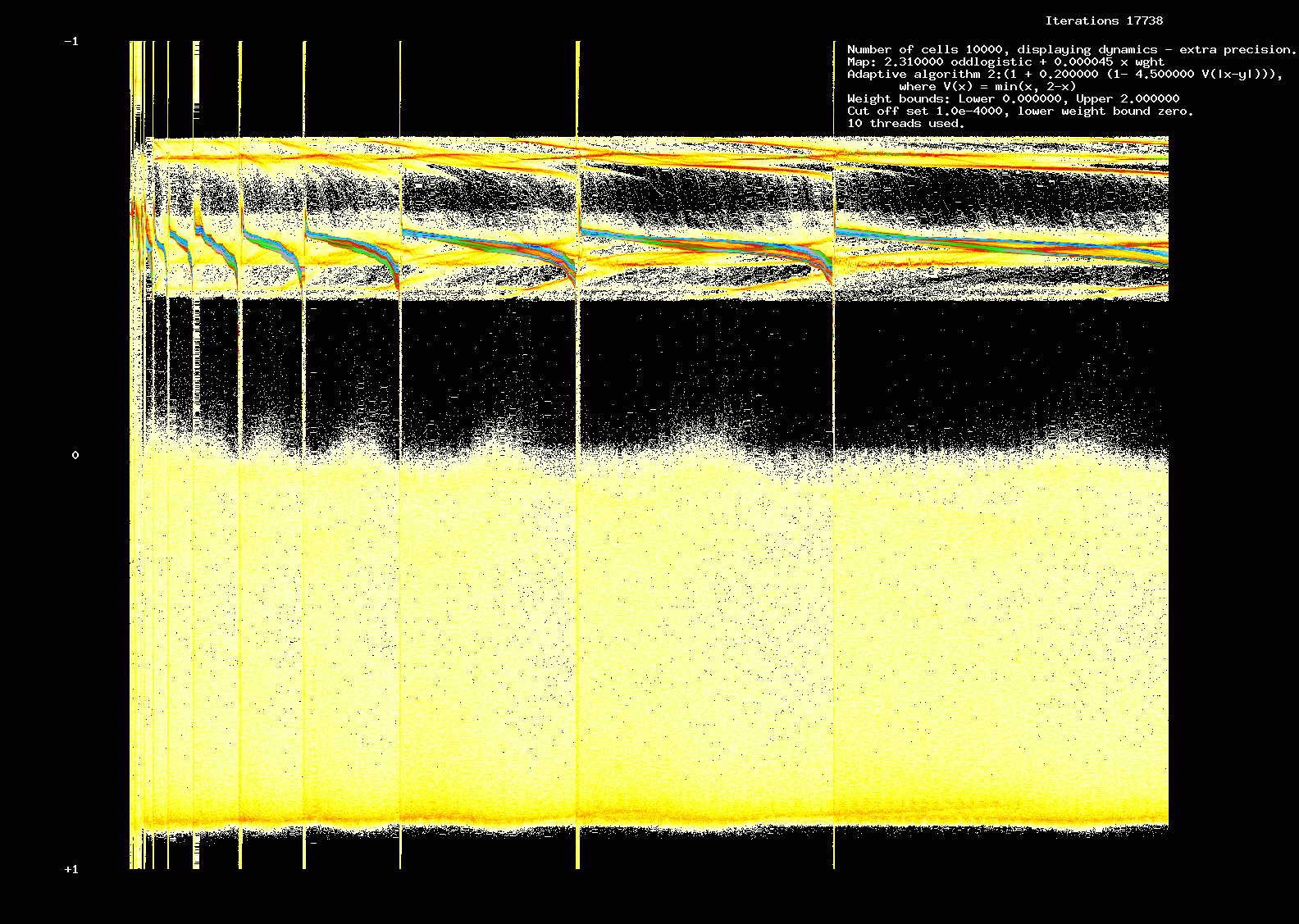After making some mistakes, we deliberately decided to mess up the global side by only synchronizing threads every hundred or so iterations (normally there are 4 or 5 synchronizations per iteration.) We call this a SLOGALS architecture (SLOppy GALS). We show the results of one such computation of 10,000 cells, 10 threads with synchronization every 200 iterations. The parameters are otherwise the same as for the simulation shown in Figure 6. Moral: providing dynamics is of right sort, and we are interested in qualitative results, we can sometimes be sloppy about the asynchronous part of the program. There is a cost: sometimes the computation will give the wrong result but it will always complete. Figure 18. Dynamics: 17,738 iterations, 10,000 cells SLOGALS architecture. Research supported by NSF Grants DMS-0600927 and DMS-0806321. Software using net programs and including some components based on ATLAS and CBLAS libraries as well as custom extra precision software. Return to Mike Field's home page. Return to Research page. Return to Networks page. Home page UCSB Department of Mechanical Engineering. email: mikefield@gmail.com Professor Mike Field Department of Mechanical Engineering University of California Santa Barbara, CA 93106