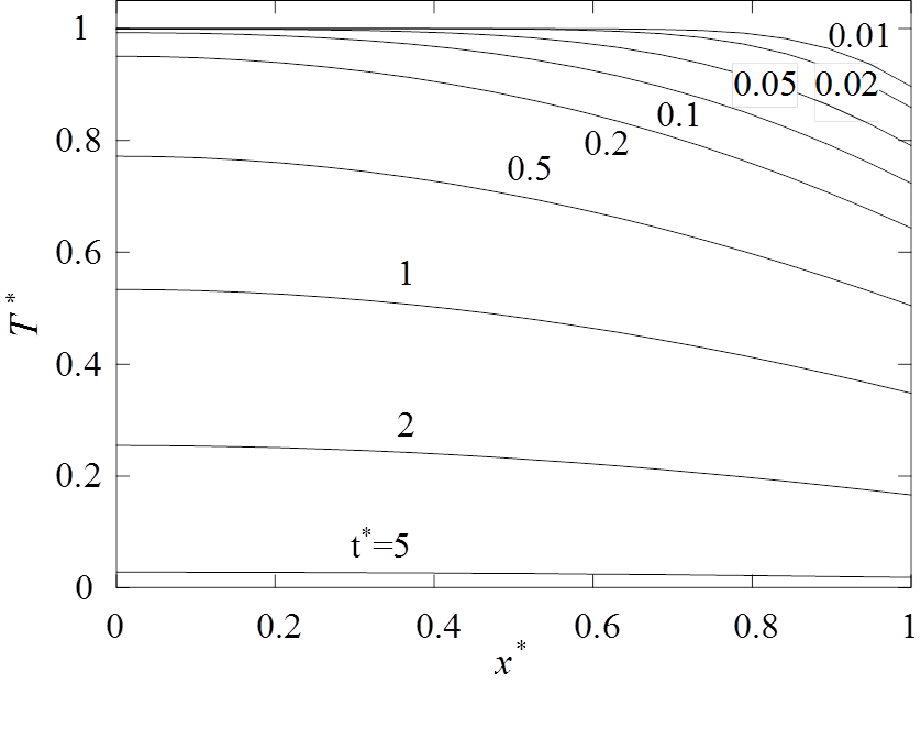
Transient slab cooling

 

The temperature profile of a slab convectively cooled through the front surface from T_o to the bath temperature T_∞ is found by separation of variables to have the solution:

where:

 

The dimensionless eigenvalues β_n are selected to satisfy the transcendental eigenvalue equation:

, for n=1,2,3 ...

 

A specified number of roots to the eigenvalue equation can be found numerically using the function Bn( )

 

Bi=1;

EigenErr = @(b)b.*sin(b)-Bi*cos(b);

EigenVal(EigenErr,7,pi)'

ans =

    0.86033    3.42562    6.43730    9.52933   12.64529   15.77128   18.90241

 

The temperature solution in the slab can be expressed by the function:

function T =Tslab(Bn,x,t)

  Cn = 4*sin(Bn)./(2*Bn+sin(2*Bn));

  Bn2 = Bn.*Bn;

  T = ( Cn.*exp(-Bn2*t) )' * cos(Bn*x);

 

To visualize the temperature solution in the slab, arrays of discrete spatial points and temporal points are defined:

x = linspace(0,1,20); % positions to evaluate T

t = [0.01, 0.02, 0.05, 0.1, 0.2, 0.5, 1, 2, 5]; % times to evaluate T

 

To calculate and plot the solution, using 100 eigenvalues in the series, the following steps are executed:

Bn=EigenVal(EigenErr,100,pi);

T=Tslab(Bn,x,t);

plot(x,T);

axis([0 1 0 1.05]);